- Home >> News >> Research Progress
Research Progress
Progress of Institute of Mechanics in Turbulent/non-Turbulent Interface Identification
Turbulent and non-turbulent (or weak-turbulent) regions coexist in many flows. Detecting the turbulent/non-turbulent interface is crucial for the development of turbulent models. In most conventional turbulent/non-turbulent interface identification methods, one quantity (such as the kinetic energy of velocity fluctuations or the vorticity intensity) is used along with a threshold value to reflect one of the characteristics of turbulent flows. Because the threshold value is specified artificially based on the experiment of the user, it is challenging for these conventional criteria to capture the characteristics of turbulence in an objective manner.
Recently, Professor Zixuan Yang et. al proposed to use the Extreme Gradient Boosting (XGBoost) method to identify the turbulent/non-turbulent interface in cylinder wake (upper panel of figure 1). The XGBoost method can treat multiple variables as the input. To avoid specifying the reference frame of coordinates, we proposed to use the invariants of the flow as the input to identify the turbulent/non-turbulent interface. According to the transport equations of important variables in turbulent flows, we choose in total 16 variables, including the kinetic energy of velocity fluctuations k and the non-trivial invariants of the mean strain-rate tensor S, mean rotation-rate tensor Ω, strain-rate tensor fluctuation Sˊ, rotation-rate tensor fluctuation Ωˊ, and second-order algebraic polynomials among them, as the input features to train the detector. The XGBoost is a supervised machine-learning method. Besides the input variables described above, the flow state needs to be given along with the training samples. Therefore, the training samples are chosen from the flow region where the flow state is known (lower panel of figure 1). Once the detector is trained, it is applied to all the discretized grid points to identify the flow state there, and as such the turbulent/non-turbulent interface is obtained as the solid line in figure 2.
Compare to the conventional methods, the proposed method based on machine learning has the following advantages. (1) The XGBoost method can treat multiple variables as the input, and (2) no threshold value needs to be specified. Therefore, the turbulent/non-turbulent interface obtained from the proposed method is believed to be more objective. Besides identifying the turbulent/non-turbulent interface, the XGBoost method can further give the importance of the input features. The more important a feature is, the more significant this feature variable between turbulent and non-turbulent flow states. Figure 2 shows the contours of the four most important features, which are, from top to bottom, the kinetic energy of velocity fluctuations k, and second invariant of tensor Sˊ· Ωˊ+Ωˊ· Sˊ, the third invariant of tensor Sˊ· Sˊ+Sˊ· Sˊ, and the second invariant of. Ω· Sˊ+Sˊ·Ω Among these variables, characterizes the unsteadiness of turbulent flow, the second invariants of Sˊ·Ωˊ+Ωˊ· Sˊ and Ω· Sˊ+S· Ω indicate that the vortex stretching is an important feature of turbulence, while the third invariant of Sˊ· Sˊ+Sˊ· Sˊ shows the three-dimensionality of the turbulent flow. It can be also seen from the figure that if any variable is used solely as the input feature, it tends to misidentify the turbulent/non-turbulent interface in some regions. For example, if the second invariant of Sˊ· Ωˊ+Ωˊ· Sˊ is used as the input, the non-turbulent flow region near the separation point on the side of the cylinder is misidentified as turbulent region.
The above work is published in Journal of Fluid Mechanics, 905: A10, 2020.
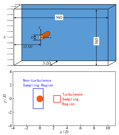
Figure 1. Sketch of the identification of turbulent/non-turbulent interface in cylinder wake. Upper panel: the computational domain of numerical simulation. Lower panel: the sampling region of the training data
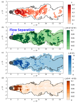
Figure 2 Turbulent/non-turbulent interface (solid line) obtained from the proposed method. The color contours show the kinetic energy of velocity fluctuations k , and second invariant of tensor Sˊ· Ωˊ+Ωˊ· Sˊ , the third invariant of tensor Sˊ· Sˊ+Sˊ· Sˊ , and the second invariant of Ω· Sˊ+Sˊ·Ω from top to bottom panels.